Autoencoder: Deep Learning Swiss Army Knife

“If you were stuck in the woods and could bring one item, what would it be?” It’s a serious question with a mostly serious answers and a long thread on quora. The very practical answer is a knife. Of course not just any knife, but all-purpose 21in1 Swiss Army Knife with a large blade, wood saw, toothpick, corkscrew, bottle opener, scissors, nail file, nail cleaner and loads of other tools that don’t look familiar at first glance. When it comes to survival in a world full of machine learning problems there is one algorithm which may be as versatile as Swiss Knife, and it is an autoencoder.

An autoencoder is a special type of neural network that takes the same values on the input and the output layers. In its simplest form, it consists of an encoder function hidden layer and decoder functionThe aim of encoder is to map input data into lower dimensional representation called code. Along with dimensionality reduction, decoding side is learnt with an objective to minimize reconstruction errorDespite of specific architecture, autoencoder is a regular feed-forward neural network that applies backpropagation algorithm to compute gradients of the loss function.

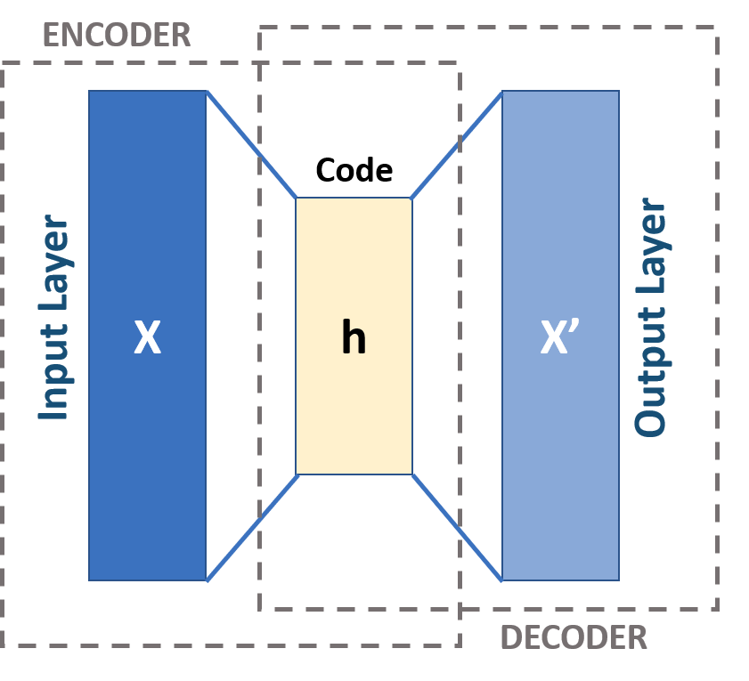Diagram of autoencoder architecture

Depending on the number of neurons in the hidden layers, there are two types of autoencoders:

undercomplete,
overcomplete.

In undercomplete autoencoder dimensionality of hidden layers is smaller than the input layer. Learning to compress high dimensional input into lower dimensional representation forces network to capture only the most important features. Opposite scenario comes into play when dealing with overcomplete autoencoder where hidden code has more neurons than the input. This type of network architecture gives the possibility of learning greater number of features, but on the other hand, it has potential to learn the identity function and become useless. One way of handling this threat is implementing regularization. Regularized autoencoder instead of preserving the encoder and decoder shallow and the code size small, uses a loss function that encourages the network to prevent from just copy its input to its output.

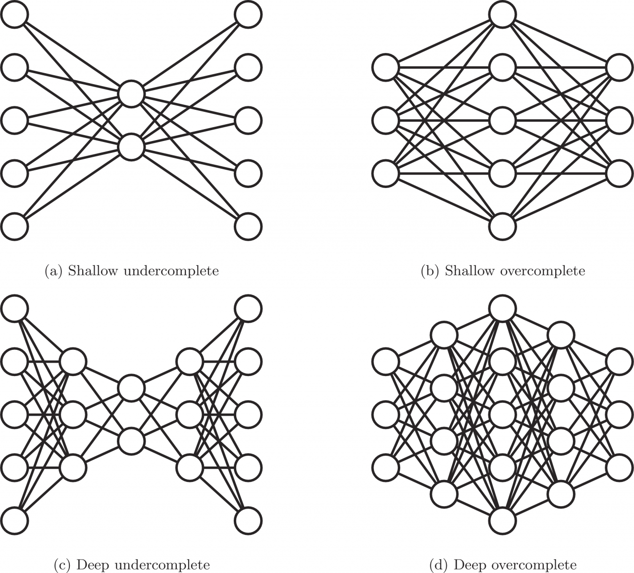Architecture of undercomplete (left) and overcomplete (right) autoencoders.

[https://www.sciencedirect.com/science/article/pii/S1566253517307844]

Autoencoders owe their recent popularity to the rapid development of unsupervised learning methods where they find their multiple applications. Large part of the latest scientific publications in the field of deep learning describes researches on various types of autoencoders and their utilization. The following paragraphs are intended to introduce versatility and use cases of autoencoders for solving common data science problems.

1in1 Dimensionality reduction

By definition autoencoders learns to represent high dimensional input into lower dimensional latent space. It’s nothing else but dimensionality reduction. The same can be achieved using for example PCA or LDA. The main advantage of autoencoders over the aforementioned algorithms is its ability to map more complex, nonlinear relationships between data. Low-dimensional features representation can improve performance on many tasks, such as classification or clustering. More compressed input means also less memory and faster runtime.

2in1 Classification

Assume that given is the problem of fraud detection in a field of behavioral biometrics. This is a typical binary classification example. Similar as in other fraud detection tasks, there is a high class imbalance due to existence of very few or none of the fraudulent observations. Fortunately, here comes the handy solution for this problem. Autoencoder can be trained on observations from only one class i.e. rich in training cases non-fraudulent class. Model built this way will learn to reconstruct normal user behaviors assigning them relatively low reconstruction error and high error for fraudulent, unknown behaviors. In case of multiclass classification problem, one way of implementing autoencoder would be to train multiple, mentioned above, one-class autoencoders and stack them at the end. Once the first stage of training is done, another classifier is built on top using reconstruction errors as input and real labels as output.

3in1 Anomaly Detection

According to Google, anomaly is “something that deviates from what is standard, normal, or expected”. The challenge and approach for dealing with anomaly detection is basically the same as in classification example explained above. By definition, anomalies occur rarely and don’t bring to many training cases. Autoencoder trained on normal observations should yield low reconstruction error when given are a new cases from typical distribution and high error for abnormous cases, since the model didn’t learn to reconstruct them well. Setting appropriate threshold on reconstruction error will allow for efficient detection of outliers.

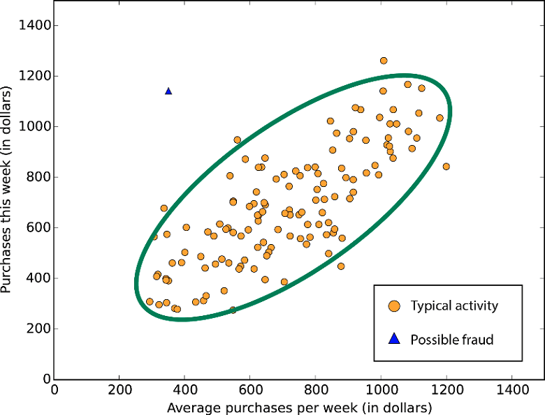Visualization of anomaly detection.

[https://www.researchgate.net/figure/Figure-1-anomaly-detection_fig1_321682378]

4in1 Clustering

Over the past few years, autoencoder implementations have been gaining more and more popularity in a field of clustering. One of the first works in this area was “Unsupervised Deep Embedding for Clustering Analysis” by Junyuan Xie, Ross Girshick and Ali Farhadi. Proposed method learns a mapping from high-dimensional data space to a lower-dimensional latent feature space in which it iteratively optimizes a clustering objective. Experiments on various implementations of deep learning clustering using autoencoders, show significant improvement over the state-of-the-art clustering methods. Cluster analysis is also a powerful tool in a field of behavioral biometrics. Users are grouped based on similarities in their behaviors. It allows to analyze groups of users rather than individuals and save computational time.

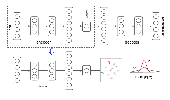
Deep Embedding Clustering network diagram. [https://arxiv.org/pdf/1511.06335.pdf]

5in1 Denoising

Autoencoders also have the ability to get rid of noise in data. For example, adding some stochastic noise to the original input images creates their corrupted version. This operation forces autoencoder to learn latent feature representation from distorted input and reconstruct image to it’s original, denoised form. Network built this way will benefit in robustness and ability of learning features from input data instead of just copying it. Denoising Autoencoders can be applied i.e. as image pre-processors in Optical Character Recognition where they improve a quality of scanned documents removing printer inks smudges or other irregularities.

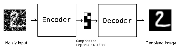
Diagram of denoising autoencoder. [https://www.pyimagesearch.com/2020/02/24/denoising-autoencoders-with-keras-tensorflow-and-deep-learning/]

6in1 Image generation

Variational Autoencoder (VAE) is one of the most promising types of autoencoder. VAE belongs to generative models like GAN’s or Boltzman machine and is particularly suitable for the task of image generation. The main difference between traditional autoencoder and its variational version lies in the approach of constructing hidden code layer. A VAE, learns to represent the input in a form of statistical distribution using mean and variance as parameters rather than a ‘fixed’ values. Distribution parameters are used to randomly sample elements. Next, decoder reconstructs those elements to their original form. Stochasticity applied in sampling process improves robustness and forces encoder to learn meaningful representations in hidden code layer. Autoencoder model created in this way allows for creating new objects by sampling and decoding from the latent feature space. VAE are commonly used for generation of images, sounds, music or texts.

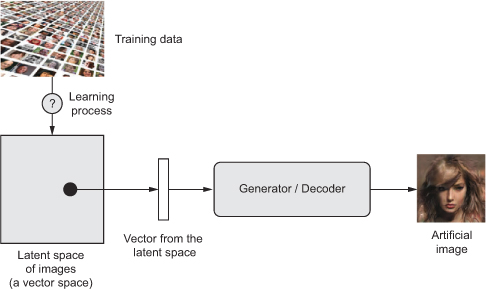
Diagram of image generation with variational autoencoders. [https://gaussian37.github.io/deep-learning-chollet-8-4/]

7in1 Information Retrieval

Other task that benefits from autoencoders ability to project data into lower-dimensions is called information retrieval (IR). IR stands for the science of searching for information in documents, finding documents itself or searching within databases. In this case, autoencoder is trained to produce low-dimensional, binary code layer. Thanks to this operation, database entries can be stored in a hash table that maps created binary code vectors to entries. This approach to information retrieval is called semantic hashing and allows for efficient searching for database entries that have the same or similar binary code as given query.

Nin1

In fact, it’s all just a piece of a broad spectrum of “Swiss Army Autoencoder” implementations. But is it really that great? Using a pocket knife metaphor, it’s not easy to find someone who cuts nails and bread with the same tool, even when it’s all-in-one swiss knife. The same applies to the autoencoder. Taking into consideration classification problem, results achieved with traditional Multilayer perceptron or gradient boosting methods like XGBoost would probably outperform autoencoders in vast majority of applications. In case of image generation, most practitioners believe in GAN’s over the Variational Autoencoders.

As any other algorithm, autoencoder also has its drawbacks like:

high complexity (especially Variational Autoencoder),
requires a lot of data,
training of the model is computationally expensive,
representing features in a latent space causes losses in interpretability,
if the test set doesn’t come from the same distribution, then ability to reconstruct the data significantly decreas,
they are prone to overfitting and therefore require regularization.

Having that in mind, there is “No Free Lunch”, and there is no algorithm that solves perfectly all machine learning problems. Almost all algorithms make some assumptions about the relationships between the predictor and target variables, introducing bias into the model. Effectiveness depends on how well those assumptions will fit to the true nature of data.

Books/papers:

Goodfellow I., Bengio Y., Courville A., “Deep Learning”, chapter 14

Chollet F., “Deep Learning with Python”

Kingama D. P., Welling M., “Auto-Encoding Variational Bayes”

Xie, J., Girshick R., Farhadi A., “Unsupervised Deep Embedding for Clustering Analysis”

Lectures:

Ng A., “Sparse autoencoder”

“Autoencoders”, Stanford

Other sources:

https://blog.keras.io/building-autoencoders-in-keras.html

https://en.wikipedia.org/wiki/Autoencoder

https://jjallaire.github.io/deep-learning-with-r-notebooks/notebooks/8.4-generating-images-with-vaes.nb.html